
Ten years ago, the shipping industry (and most other industries for that matter) participants came to the realisation that it was going to be affected greatly by data, data capturing, data analytics and subsequently data driven decision making. However, as is many times the case with large disrupting events, the details on how it would be affected, how data was to be used, was not clear, neither was the timeline.
Today, some 30 years since the first use of the term Big Data. The data series that we are currently gathering in relation to shipping, is so large and complex that it cannot be analysed, managed or sometimes even handled by humans. A small pocket of stronger demand for freight or a small section with an oversupply of tonnage causes ripples through the market. This makes the breadth and diversity of information that can and should be used in picking signals very large. Even when looking at small markets, with small number of factors involved, like a single cargo route, one can no longer digest and manage all the available data in a way that it can help make an educated guess.
However, it appears to many that we are still witnessing the commencement of the data disruption cycle. This view is shared amongst those that are seeing the increasingly accurate outputs of the machine learning models. Apart from a plethora of primary data, i.e. AIS data, fuel consumption, commodity prices, bunker prices, commodity spreads between locations etc, we are starting to have what can be coined as “new data” or perhaps derived data. This is forecast data that is the output of Machine Learning models (ML) that can be used by other ML models to forecast other values and so on.
Training a Supply and Demand ML model using historical Ballast vessels in order to forecast the available tonnage in an area 3 weeks from now was optimal until very recently. However, we can now feed it Ballast vessel number forecasts that are being produced by other ML models whose accuracy we can quantify and measure. Same goes for Soybean crush spread, bunker price etc. The more accurate the models become in forecasting, the more information and data we have to feed the other models that use their outputs as driver inputs.
In addition to the “new data”, we also have new primary data being produced by new technologies, like satellite image reconstruction of stockpiles on docks. Colour analysis of satellite data determining the maturity and quantity of field crops and subsequently volume and timing of harvest, real-time vessel engine rpm, weather data, intraday FFA clearing prices and so on.
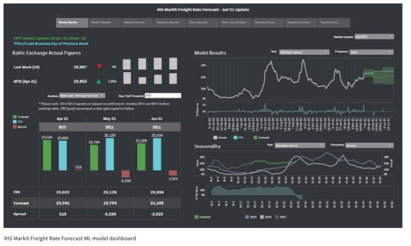
These vast quantities of data are optimally handled by ML models, linear models etc with measurable accuracy. The reason we know this, is because we are comparing their results with the results of humans. The forward markets are the amalgamation of the level the market participants are willing to transact. We know the ML models are getting better because their accuracy in forecasting the future state of the market is superior to the “forecast” of the market participants themselves, the futures market.
The fact that the ML models are better forecasters than the futures financial market brings up more uses and more applications in this very volatile market. If one has a more accurate curve than the forward curve itself then the FFA curve is only used as a means of marking the potential close out of my existing position to market or my ability to hedge a forward position. If I want to make more realistic decisions on the potential outcome of the forward market, then the ML model results and forward curves are more useful. This applies to Sale and Purchase decisions of vessels, Financial Cash flow evaluations, NPVs, Long term Time Chartering decisions, tonne mile Mining feasibility studies, shipping loan portfolio management etc.
The fact that a Shipping or Cargo Trader may now have an ML driven proprietary curve is nothing new. In the late 90s and even today Treasury departments throughout most big banks had their own internal curves that they used to mark their book to market for internal purposes. Traders used to say that they were different from Libor or other external price discovery mechanisms mainly to reflect liquidity. The data driven Proprietary curves produced by the ML models may do just that. The only difference is that the ML models are forecasting liquidity not just in the execution of the derivative or the fixture itself but rather the condition of all other drivers that determine the price. The data driven model can make realistic assumptions on the depth of the market, after all we now have FFA intraday prices amongst others.
Applying ML models in managing Freight market exposure
Some initial application examples indicate that the machine learning models don’t need to reach a high level of accuracy to achieve great results on fixing ships/ cargos and hedging of Freight Market exposure. This is mainly because shipping is an averages game and so are the ML model results. When a fleet of vessels or a cargo book is exposed to the market in a series of small increments of risk, such as cargo stems and vessel spot fixtures, the manager needs to get enough of them right and make sure that the total return from the right ones is higher than the not so successful ones. This is very similar to Equity portfolio management. One manager can look
for ways to beat the S&P500 because they can hold many stocks, not all have to provide superior results, just enough will suffice for the purposes. In addition, a manager can trade the trends and momentum for small periods of time. We all know what has happened to manual stock-picking and how smart beta data driven algorithmic trading has eclipsed traditional management. This appears to be happening to shipping, and it affects both execution, fleet management and cargo exposure management.
The main reason for the success is because ML models need to be good on average or their signals can be applied in specific higher tolerance parts of the Chartering/Hedging workflow. Out of the 10-12 or so spot fixtures of a Capesize Vessel in the last 12 months, fixing it for a longer period just twice (when ML model indicates) leads to beating the generic spot fixing by over 7% (fix 40 day business instead of 30), so offering a greater ability to beat the Baltic Index, especially on a portfolio basis. These results when applied to a fleet could be pushed higher subject to risk appetite.
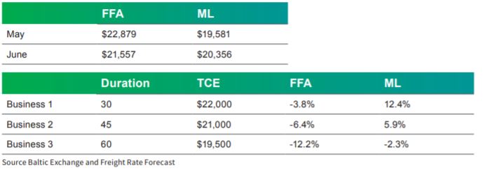
The ML models appear to be back testing well also in the management of the nearby exposure of freight. When one is evaluating potential spot business for a vessel’s next fixture, they get a completely different evaluation and perspective when using the FFA and when using the ML forecast:
Business 1 has a duration of 30 days and a Time Charter Equivalent of $22,000. When it is marked to market using the FFA curve it appears to be almost 4% below the Index, however when marked to market with the ML model forecasted curve it appears to be beating the Baltic Index by almost 13%. The business that appears to be capturing revenue above the Baltic Index when evaluated using the FFA curve for a Shipowner (or savings for a Cargo trader) is actually losing him/her money. The existence of the ML model curves changes the
way potential business is evaluated. It also affects the marking to market of the nearby of the Cargo or Fleet portfolio in its entirety. The difference in the evaluation of the potential business also applies to the existing committed business, so a fleet that looks like its capturing revenue above Index may actually be failing to do so. It is this very nature of small decisions of small exposures of one’s business to the market risk that make the ML models so successful in the Shipping business.
If a Machine Learning model forecasts correctly the trend (irrespective of the level) in the Dollar per Ton price of a Route or the trend of the Average Time Charter Index, a Charterer/Grain Trader can take the longer/ shorter spot business, or he/she can take the said business unhedged, or even take a small leveraged risk on the FFA market. The implications to a Fleet or a Cargo book are significant. Similar applications exist when applying ML and linear model signals on hedging one’s forward market exposure using averages, it is highly successful in calibrating future income within management set bounds. The applications of the good quality driven signals have numerous applications depending on one’s market exposure. One could postpone cover; another can postpone execution and so on. The possibilities in applying ML models to shipping are numerous. That is until we get to the point that we cover all possible uses and all possible decisions. This most likely means we have arrived at the self-fixing, self-managing fleet, self-executing cargo book.
Why is it that its easy? Is it because this is an unsophisticated market? Is it because the Demand and Supply equations are simple? Is it because the ML model requires expensive data to get to a usable level of prediction accuracy, (cost may be a barrier to entry). One potential explanation is that applying the new ML forecasting technology in workflow/execution has not been done yet by enough players to make it non-profitable.
In addition, the means of applying and incorporating into one’s business model is highly specific and the participants in the Freight market have numerous business models and objectives.
What is clear is that the achievement of optimal Hire for Vessels, Trading Cargoes and even FFA’s is becoming data driven. It appears imperative to incorporate data driven decisions into one’s execution, hedging, evaluation, benchmarking etc. It is a case of the early adopter in the disruption placing themselves better in the developments that are to come. Only the players that spend the time to incorporate data driven decisions, apply the signals to their trading and risk appetite, add the ML nuances into their workflow will benefit from the improvements in the models as they are being developed and improved.
Source: IHS Markit


